Huff(man)ing and Puffing - Huffman Image Compression
Morgan McGuire and Thomas P. Murtagh
Williams College
| Summary |
Huff(man)ing and Puffing --
A project composed of three laboratory assignments that explores aspects of image
processing that culminates in an experimental evaluation of several
Huffman-code based image compression schemes.
|
Topics
|
All three laboratory assignments are primarily focused on
developing skills in array processing. In addition, the second assignment explores inheritance,
and the final assignment involves a recursive algorithm.
|
Audience
|
Appropriate for the end of CS 1 or beginning of CS 2.
|
Difficulty
|
The assignments for the three weeks of this
project are respectively introductory, intermediate, and advanced.
|
Strengths
|
The strength of this project is that it simultaneously teaches programming,
algorithm design, and scientific methodology. Students build an experimental tool
using a broad spectrum of array techniques. It combines image processing (which
students love) with an scientific/experimental twist (which instructors love).
|
Weaknesses
|
- The complete project would occupy several weeks
of course laboratory time.
- The project depends on SImage, a non-standard class for representing images.
(It also depends on a second
non-standard class for GUI event handling, but this
dependence could easily be eliminated as discussed below.)
|
Dependencies
|
All of the weekly assignments
require knowledge of basic
control structures, class and method definitions, and the construction
of simple Swing GUI interfaces. The last two assignments assume that
the students have familiarity with arrays. The last assignment assumes
knowledge of recursive methods and requires that some class time be
devoted to the explanation of Huffman codes.
|
Variants
|
We use these three assignments in conjunction with lecture presentations that
overlap with the project as part of
an integrated introduction to array processing. With some care, one could
replace one or both of the first two steps of the project with other labs
that develop array processing skills and then use the last week of our
series of labs as an independent exercise.
|
A Multi-week Image Processing Project
For years, each of the exercises in our CS1 course were completed in a single week independent of
all of the other exercises. The assignment described here, on the other hand, is one of a
series of multi-week projects we have designed as part of a
revision of our CS1.
There are clear advantages to assigning projects that are longer than one week. With the extra time,
it is possible for students to tackle problems that are more interesting and to produce
final products that better satisfy their creative impulses. These larger projects also make it
easier to expose students to design issues during the first course. Finally, it gives students
more time to develop fundamental skills by amortizing over multiple weeks the overhead required to
learn the context for the problem.
There are, however, several obstacles to using multi-week assignments in CS1. Given the pace
at which new programming techniques are typically introduced in CS1, any single handout that
described a two or three week project would probably describe aspects of the project
requiring programming skills the students would not acquire
until some time in the midst of working on the project. There is also the issue of
compounding failure. If a student gets stuck on one of the early steps of the project,
they could easily fall critically behind as the deadline for the complete project
approaches.
With these issues in mind, we have designed our multi-week projects, including the one
described here, as a series of tightly integrated, single-week assignments. The students
receive a new lab handout each week. The handout describes a program the students
should complete as an independently useful application
whose construction only requires skills they have already learned.
From the instructor's perspective, however, the
modules of the programs completed in the early weeks of a project are designed
to build upon one another, eventually serving as components of the larger program
produced in the last week of the project.
The project described here leads the students to construct an image processing
program that is eventually used to experiment with the effectiveness of
a number of image compression techniques. The assignment begins with simple
manipulations, such as those available in the popular Photoshop image editing software.
These are applied to specially prepared images to yield fun surprises when the students
have a correct implementation. The tail of the assignment uses the same building blocks
as today's real compression algorithms. However, as can be seen in the lab
handouts linked below, the word "compression" does not even appear in any of the
lab materials until the last week. As a result, while we view the three
assignments described below as part of a single project, others could
choose to adopt just one or two of the labs as assignments.
Step 1: Pixel Brightness Value Manipulation
 For the first week of this project, the students produce a program that allows them
to load image files and then alter the images by either scaling the brightness
values of all of the pixels in the image, or
by reducing the number of distinct values used to represent brightnesses,
effectively reducing the number of colors used to present the image.
For the first week of this project, the students produce a program that allows them
to load image files and then alter the images by either scaling the brightness
values of all of the pixels in the image, or
by reducing the number of distinct values used to represent brightnesses,
effectively reducing the number of colors used to present the image.
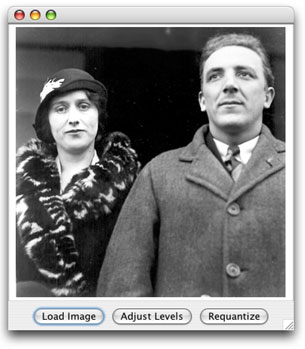
A snapshot of the program's main window is shown on the right. The interface
provides three buttons. Pressing the "Load Image" button displays a dialog
box that can be used to select the image displayed in the window. Pressing either
of the other two buttons creates a new window in which one of the two forms
of adjustment described above can be performed.
For example, pressing the "Requantize" button would make the window shown
on the left appear. In this window, the slider at the bottom is set to
the value 2 (which is displayed to the right of the image), indicating that only
two distinct brightness values should be used to display the image.
|
You can experiment with this program or either of the programs we ask students
to construct in the following two weeks of this project by downloading our
archive of sample image processing lab solutions.
When unpacked, this archive should produce a folder containing four .jar files
and a sub-folder of sample images.
The .jar files named Step1Solution.jar, Step2Solution.jar, and Step3Solution.jar
are executable and correspond to the programs the students are asked to produce
during the three weeks of the project. For example, to run the lab from the first
week, you would double-click on Step1Solution.jar. Once the program window
appears, click on the "Load Image" button and navigate into the AllImages
folder in the same folder to select an image to manipulate.
The squintV2.8.jar file contains the small library of classes this project
depends upon. The library is called Squint.
This project only depends on the GUIManager and SImage classes
from the library. Click here for
complete documentation of the Squint library.
The dependency of these exercises on the Squint library can be easily reduced to
the use of the single SImage class. Students will need to be familiar with
some mechanism to create a GUI interface in order to complete these labs.
In our course, students learn how to do this using Squint. Others might
teach their students how to create GUIs using only standard Swing classes
or using the classes in the ACM Java Task Force
libraries. These lab could easily be adapted to replace the use of the
Squint GUIManager class with either of these other libraries.
|
The lab handout for the first week of the project reflects
another unusual aspect of many of our labs. While in the past we made sure
to discuss each programming technique in class before we would
expect students to use it in lab, we now often give students a first exposure
to a new technique in lab. Then, we take advantage of the practical experience
students have gained in lab to provide a more effective general introduction
to the new topic in class. The topics introduced in this lab are arrays
and array indexing. Our students have no previous introduction to arrays
before completing the lab. As a result, the handout is written
more as a tutorial than our typical lab handouts.
From our point of view as instructors, it is the tutorial nature of this lab
that makes it nifty. Who would ever guess that students could learn arrays
on their own? In particular, who would guess that they could learn arrays on
their own by learning "more complex" 2D arrays before 1D arrays? Luckily,
the connection
between what they already know about cartesian coordinates and the way subscripts
are used to select pixels is strong enough that students handle this without
great difficulty, and after this lab,
they come to class well prepared to learn more general ways
to use arrays.
From the point of view of our students, this lab is nifty because it is
their first change to manipulate images. The visual feedback is
very satisfying to them.
Step 2: Pixel Brightness Value Manipulation
Both of the imaging operations that students implement in the first week involve only
simple array operations. They write two sets of nested loops that
apply a given formula independently to all of the pixel brightness
values in a 2D array. In the second week, we seek to expand
the set of techniques used to include 1D arrays, loops to find
minimum and maximum values, and operations that combine values from
several positions in an array or from different arrays.
The interface for the program the students are asked to complete in the
second week of the project is shown below.
 The interface allows a user to manipulate two images at the same time,
one on the left side of the program window and the other on the right.
Independent controls are provided for each image. Some of these
controls repeat the functionality from the first lab and are implemented
using the same code (e.g., the "Brightness levels" slider performs the "Requantize"
function).
The interface allows a user to manipulate two images at the same time,
one on the left side of the program window and the other on the right.
Independent controls are provided for each image. Some of these
controls repeat the functionality from the first lab and are implemented
using the same code (e.g., the "Brightness levels" slider performs the "Requantize"
function).
There
are several new controls present on both the left and right panels. The user can
save a modified image. By adjusting the "Block Size" slider the user can
change the spatial resolution of the image displayed. In the snapshot
above, the setting of the right "Block size" slider results in an image in
which each pixel has been replaced by the average brightness
of a 6x6 block of pixels.
The "Show Histogram" button causes the program to display a histogram of the
brightness values in a separate window as shown on the right. The "Expand
Range" button causes the program to scale the brightness values so that
they extend through the full range from 0 to 255. This requires first
finding the minimum and maximum brightness values in the original image.
 In addition, there are several controls at the bottom of the window that
provide for interactions between the two images displayed. "Move Left-> Right"
simply replaces the image on the right with the image on the left while
"Insert Left-> Right" pastes a copy of the left image over the right image.
The "Show difference" button displays an image whose brightness values
are determined by computing the differences between corresponding pixels
in the images on the left and right. A snapshot of such an image is shown
on the left. The details of all of these operations are described in
the lab handout for week 2 of the project.
In addition, there are several controls at the bottom of the window that
provide for interactions between the two images displayed. "Move Left-> Right"
simply replaces the image on the right with the image on the left while
"Insert Left-> Right" pastes a copy of the left image over the right image.
The "Show difference" button displays an image whose brightness values
are determined by computing the differences between corresponding pixels
in the images on the left and right. A snapshot of such an image is shown
on the left. The details of all of these operations are described in
the lab handout for week 2 of the project.
Completing this assignment clearly provides the students with ample
opportunity to exercise their knowledge of arrays. The block
averaging and image differencing operations require them to combine
information from different entries of arrays in interesting ways.
Building the array of histogram values and finding the minimum and
maximum values gives practice with 1D arrays.
For students, the "nifty" in this assignment comes from some of the
surprising results of applying the operations they implement.
Basically, the sample images we provide are rigged to make these
transformations interesting.
For example, if one loads the image
file "grifSecret.gif", a picture of Griffin Hall,
the stately campus building shown in the snapshot of the program's
interface above,
copies it to the right, changes the copy to be displayed using only
16 brightness levels and then presses "Show Difference", an image like the
one on the right appears. Not very interesing!
If, however, you then press
"Expand Range", the image changes dramatically to appear like the image
shown below displaying an aerial view of the pentagon
(perhaps encouraging the Homeland Security Department to visit your lab!).
The original image is an example of steganography. The brightness
values for the image of the Pentagon are hidden in the low-order bits
of the brightness values of the image of Griffin Hall.
There are several other such surprises in the collection of image file
provided with our lab materials.
All of the images in the "ExpandRange" folder reveal interesting images
when the "Expand Range" operation is applied. "There be dragons" (well,
at least one) in the 10x10.png image found in the "Average" folder if
you change its block size to 10.
Computing the difference of the two nearly identical images in the
"Difference" folder yields a Halloween treat. (Guess when we first assigned
this lab!)
Starter code
Above, we mentioned that one risk of having a multi-week project in a
CS1 course is that students who fall behind early might never catch
up. The obvious way to deal with this is to provide students with
a solution for week N's work as they begin week N+1. We take a slight
variation on this approach. We provide all of the students with
starter code in week N+1 that is similar enough to what they completed
in week N to make it easy for them to understand but different enough
that all students are expected to use the starter code rather than
what they produced the preceding week. This way, at the end of the
project, everyone who does well throughout the project feels like
they wrote "the whole thing" because they realize they could
have easily adapted their code instead of using the starter code.
On the other hand, students who have a bad week don't fall behind.
Step 3: Evaluating Image Compression Techniques
During the final week of this project, students write a program that allows them
to measure the effect of applying several compressing techniques to images.
Then, we ask them to write a lab report describing the results they obtain.
We do two things in lecture to prepare for this exercise. First, we
explain the basics of Huffman codes. This is a topic we include
fairly early in the course to show students an example of an interesting
algorithm and to get them thinking about issues of data representation.
When we present Huffman codes, they know very little about Java programming.
They don't implement any part of the algorithm early in the course.
They just solve homework problems drawing Huffman trees on paper to
compress short text messages.
In lecture, after the students complete step 2 of the project,
we point out how many bits it takes to encode even a relatively
small image and ask if they can see any way to reduce the number of bits
required. With a bit of luck, some of them remember Huffman codes and
suggest applying them to images. Unfortunately, the naive scheme
does not work very well. The distribution of brightness values in most
images is too uniform for Huffman codes to be efficient. Using the program
they completed for week 2, however, we can demonstrate an effective alternative.
If you examine the histogram of an image produced by computing the
difference between an image and a "block averaged" version of the same
image, the distribution is far from uniform. Huffman coding this difference
image can be quite effective. Thus, we propose the following scheme
for compressing images. Compute a 4x4 block average of the original.
This image should take about 1/16th as many bits as the original.
Compute the difference between the original and the block average.
Huffman coding the difference image often gives 50% compression. Together,
the differences and the block averages encode all of the original information
at a fraction of the original size.
For the lab, we then give them a handout describing several other
such schemes and ask them to measure the effectiveness of these schemes
on a collection of sample images. Some of the schemes are lossy, so this
involves both measuring compression ratios and subjectively evaluating
image quality.
A snapshot of the interface for the program they write is shown below.
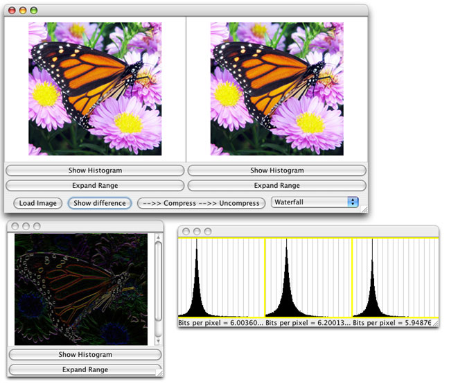
The image loaded on the left side of the main window is the image to be compressed. The
menu in the lower right corner of the window is used to select the scheme to be
applied, "Waterfall" in this case. All of the schemes are described in
the lab handout for the third week of this project.
When the user presses the "-->> Compress -->> Uncompress" button, the scheme selected is
applied to the image, a new window like that shown on the left below the main window
is displayed showing the revised representation
of the image, and the result
of undoing the transformation is displayed on the right side of the main window.
If one then presses the "Show Histogram" button in the window displaying the
revised representation, the program displays histograms of the red, green and blue
brightness components along with a figure for the number of bits per pixel
required to store this representation using a Huffman code.
Implementing this program requires implementing interesting algorithms involving both
single and two dimensional arrays. This includes implementing part of Huffman's algorithm.
Surprisingly, the part of Huffman's algorithm that the students
implement does not involve any tree data structures.
Instead, it has a great deal in common with selection sort. In the standard description
of Huffman coding, one builds larger and larger trees by repeatedly combining the
two trees corresponding to the smallest occurrence counts or occurrence frequencies.
If all one wants to do is determine how many bits are required to encode a message
rather than actually determining the exact form of the encode message, keeping
track of the trees becomes unnecessary. As a result, the algorithm the students
implement (following the description in the handout) involve repeatedly replacing
the two smallest numbers in a list with their sum.
Summary
By the end of the three weeks of this project, students have covered quite a bit of
territory. In terms of programming skills, they have learned techniques for constructing
and processing 1 and 2 dimensional arrays ranging from using simple nested loops to
process individual elements, to the application of the wavelet decomposition that
requires them to recursively subdivide and them combine the contents of an array.
In between, they encounter basic techniques including accumulating the sum of a
set of array elements, finding minima and maxima, and rotating the elements of a 2D array.
They also encounter a number of interesting algorithms and data representation schemes
including Huffman encoding, steganography, histograms, and the use of wavelets in
image processing. Perhaps most importantly, the experimental component of the
lab exposes them to the issue of evaluating the effectiveness of algorithms and
data structures used to solve a particular problem.
Additional Resources
Extra info about this assignment: